Crop production model.

We use a specific crop production model [6][7], calibrated by data which have been collected by E. Denisenko in the course of two periods: 1978 and 1983. A model structure is shown in Fig. 2.

  
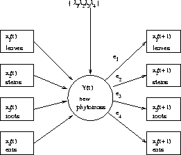
Figure 2: Conceptual diagram of the crop model. Environmental (weather) parameters: is the daily PAR, is a parameter of water regime, is the CO concentration in the atmosphere, is the daily temperature.

The basic state variables are the phytomasses of leaves, steams, roots and generative organs (ears), correspondingly. All these values are functions of time, , measured in days. The general equations of the model are:
 
where the daily net production, Y, depends both on the state variables and the weather parameters . Here is a daily amount of the photosynthetically active radiation (PAR). The latter is presented in the form of so-called solar hours. is the parameter determining the water regime of barley crops. In fact, this value depends on precipitation dynamics, in particular, on alteration and lengths of so-called ``dry'' and ``wet'' series, that is, series of days with no precipitation and days with significant precipitation without dry period between them. The parameters and are the concentration of atmospheric CO and the daily temperature.

The function Y is defined by standard dependencies taken from plant physiology and ecology (see, for instance, [8]). The coefficients , i=1,2,3,4 () describe some allocation principle, that is, they show how the new phytomass is allocated among different organs of plant. In order to calculate them we postulate the following local variational principle which reflects the process of plant adaptation to variations of environment.

All the vegetation period is divided into two parts: before and after the appearance of generative organs.

Before:

the new phytomass is allocated among leaves, steam and roots in this way that to maximise the growth rate of total phytomass in the next time, under the condition that the state of environment does not change.

After:

the new phytomass is allocated among leaves, steams, roots and generative organs in this way that to maximise the growth rate of generative organs in the next time, under the condition that the state of environment does not change.

The comparison of the model results and observed data for 1983 is shown in Fig. 3.

  
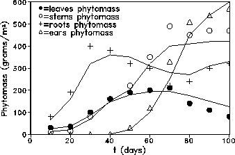
Figure 3: Comparison of the observed (markers) and model (lines) data of the Kursk region for the year 1983.

It is obvious that the crop yield , where k is an empirical coefficient and is the end of the vegetation period. In this model the crop yield is a functional that depends on the trajectories of the daily temperature, precipitation and PAR during the vegetation period. It is obvious that the -set, that is, the set of climatic parameters (climates) is a functional space, the elements of which are trajectories of the values mentioned above. In order to estimate the dependence of crop production on this type of trajectories for the future changed climate we have to know how to generate them. For this we have used a so-called