3. Parallelization of REMO
3.1 The Parallel Programming Model
The parallelization strategy based on the parallelization approach used for the EM/DM, the 2D domain decomposition. Every processor sets up its partial problem by specifying the local data structures and initializing organizational variables. In principle every subdomain can be considered as a small region running its own model. The parallelization of the different parts of the adiabatic model for the EM/DM is described in [1]. Only the organization of the I/O management is an exceptional case. There are processor groups with different task specifications. These processors are working code parallel.
For the practical implementation we chose the MPI as a portable message-passing library. All MPI - and I/O - processes are written in C and are concentrated in separate subroutines. The clear dividing line between these subroutines and hardware independent subroutines provides an easy way to manage different hardware architecture features.
For processor communications we use nonblocking send and blocking receive MPI subroutines. Nonblocking send means that the I/O operation is only initialized and there is no need to wait for it to end. This causes less waiting time, the processor can continue its computation. Of course, the sending array is not reusable until the end of the send operation. In practice this problem is solved by creating barriers for all processors after common communication points.
The time measurement was realized by using subroutines of the Fortran 90 library, namely rtc -- a subroutine for wall clock time (also real time) -- and etime -- a subroutine for user elapsed time (also CPU time). The implementation of the communication subsystem library used was the User Space (US) communication subsystem (the hardware is configured with its high-performance switch feature).
3.2 Parallel I/O Organization
In REMO a huge amount of data is necessary for input as well as for output. For a 24 hour prediction in our actual model area (193 x 121 gridpoints, 20 vertical levels) the transfer of about 28 MB input data and 48 MB output data has to be realized. Additionally there is the choice to write restart files (180 MB). The prediction period reaches up to five years. These facts underline the importance of a good parallel I/O organization to ensure a reasonable speed-up of the whole model.
Every processor of the IBM RS/6000 SP has its own operating system and is able to perform I/O operations. In operational use of REMO it is necessary to distribute the initial data fields and the boundary data fields produced by a global climate model to all processors corresponding to their subdomains. Furthermore it is necessary to write result output files, in our case typically every six hours.
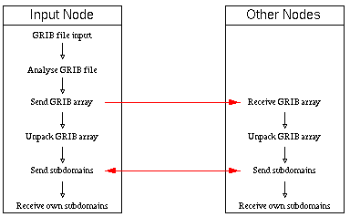
Our model input files are given as binary packed records in the GRIB (gridded binary) format. That means that a processor cannot get its data from disk space in a direct way. At first it is necessary to analyse the structure of the GRIB file and later to decode this GRIB file to build up input arrays. Therefore, only a single node (input node, generally node zero) reads the whole GRIB file to its local memory. This node analyses the GRIB structure and sends single, but complete, GRIB fields to the other nodes which then are able to unpack the fields. After decoding every node distributes the data to all other nodes according to their subdomains. Then it returns a message to the input node that it is ready for receiving new unpacked arrays. If such a message is not present for the input node it also starts decoding GRIB fields and distributing them to the subdomains. But for the input node the distribution of GRIB data to the other nodes has a higher priority. After decoding of the whole GRIB file every node has completed its own input. The tasks of the input node and the other nodes are represented in Figure 1, "Tasks of input node and other nodes".
|
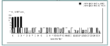
In the case of a small number of nodes this approach ensures a balanced distribution of user elapsed time, but for a higher number of nodes the load of the processors becomes more imbalanced. Figure 2, "Distribution of user elapsed time for initial data input processing" shows the distribution of user elapsed time for 4 processor nodes and for 32 processor nodes in the case of the input of the GRIB code initial data (including 120 GRIB data arrays).
Figure 2: Distribution of user elapsed time for initial data input processing |
When using a higher number of nodes a reason for a higher degree of imbalancing is the increasing impossibility of distributing all GRIB data arrays even to all processors.
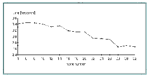
Figure 3, "Wall clock time for initial data processing" shows the wall clock time for different numbers of processors in the case of initial data processing (6,7 MB input data).
The maximum degree of parallelization depends on the number of GRIB data arrays. The unpacking subroutines themselves were not parallelized and it is not intended to do so. It is our aim to avoid GRIB input files in the future by changing the preprocessing.
The model output consists of the calculated fields and of the restart data.
Three output possibilities exist for these files:
Output of binary files using a C subroutine.
Output of binary, unformatted files using a Fortran subroutine.
Output of binary GRIB files.
On the IBM RS6000/SP we prefer writing output files with C subroutines. It is the most efficient output method in UNIX operating systems and very simple to manage. No processor communication is necessary. Every node performs its own output and can go on working.
The problem then is that the output disk space does not contain the complete model area files but only node dependent subdomains of these arrays. Therefore, after the writing of all output files every node creates a new child process (fork subroutine) and this child process then starts a program (execlp subroutine) for collecting the different parts of an array. Later these arrays will be dumped on a Tapelibrary 3494 with six drives. This sequence of output processing is not simply a transfer of work to post processing. The child process works together with the parent process in time sharing mode. That guarantees a better use of system resources, e.g. by overlapping of processor time and I/O time. The Tapelibrary dumps and compresses created files without also making any demands of processor resources.
The writing of output files with Fortran subroutines is done in the same way. The difference between binary Fortran files and binary C files is a different internal file structure. The output as GRIB files ensures compatibility with Cray users. This output is realized in a similar way to the input of GRIB files, but in reverse mode. The GRIB code output, like the GRIB code input is unsuitable for use by parallel file systems. But our current I/O approach supports also later use of parallel file systems without extensive modifications.
3.3 Dependence of load imbalances concerning different subdomain decomposition approaches
All area dimensioning parameters are defined in a separate control file. Therefore, these parameters can be changed in a very easy way without recompiling of any model source code. Before the model starts it is necessary to set different POE (partition manager) environment variables. These variables enable the specifications of such options as an input or output host file, methods of node allocation and processor count.
After the model starts every node is able to compute its own subdomain. Assuming a grid with N processors, where N = NX * NY , it is possible by variation of NX (number of processors in east-west direction) and NY (number of processors in north-south direction) to ensure an optimal result for different model areas concerning the computing time. It was our aim to investigate whether this way is suitable to obtain an acceptable load balance between all nodes without extensive source code modifications and enhancement of communication time. Two groups of load imbalances exist:
Static load imbalances
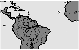
The impossibility to create in every case absolutely identical subdomains for all single node causes load imbalances in the explicit Eulerian time-step and the semi-implicit corrections. Furthermore, the surface data are concentrated over the continents only which causes an irregular grid point distribution (see Figure 4, "Investigated model area").
Dynamic load imbalances
Many other sources for load imbalances are located in the physical part of REMO, above all in the computation of radiation and convection.
Our approach is a static one, it is not very well suited to handle dynamic load imbalances. The first test variant is a square domain decomposition (e.g. NX = 4, NY = 4) , the second test variant is a rectangular domain decomposition over complete latitudes (e.g. NX = 1, NY = 16). Mainly our model area covers the area of South America and the Southern Atlantic (193 longitudes, 121 latitudes, see Figure 4, "Investigated model area").
Figure 4: Investigated model area |
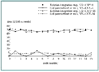
The results shown in Figure 5, "Distribution of user elapsed time for Eulerian integration and soil parametrization" illustrate the influence of these decompositions on the distribution of the user elapsed time for soil parametrization and for Eulerian integration.
Figure 5: Distribution of user elapsed time for Eulerian integration and soil parametrization |
In the case of soil parametrization the square domain decomposition provides a very bad balance between different processors. This result was expected (see soil distribution in Figure 4, "Investigated model area"). Splitting up subdomains by distributing only latitudes to different nodes results in a much better balancing of elapsed time.
These facts do not apply to the Eulerian time step. The elapsed time distribution between processors is much more homogeneous generally. An explanation for the differences are the facts that the subdomains are not absolute identical and that the boundary lines of the total domain are treated differently in the algorithms than the grid points in the interior of the domain.
Because soil parametrization is less time consuming it follows that in the case of rectangular decomposition increasing time of Eulerian integration and the decreasing time of soil parametrization cancel each other out.
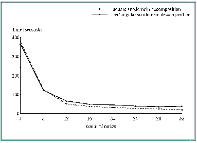
Finally a square decomposition provides better results than a rectangular decomposition. Figure 7, "Scalability of a full prediction step" illustrates this fact. So we prefer a processor distribution which approximates a square decomposition. In this way only a best possible subdomain decomposition for the Eulerian integration scheme decides the issue.
Figure 7 and Figure 6 show the scalability of a full prediction step of REMO in the case of square decomposition and in the case of rectangular decomposition by use of up to 32 processors. The measured prediction step contains the Eulerian integration scheme, semi-implicit corrections, soil parametrization, radiation and convection. It is not representative for all prediction steps, because, e.g. the radiation is computed only every eighteenth time step.
From Figure 7 it can be seen that there is a superlinear speedup going from 4 to 12 processors. The reason for this is the memory requirement of the model.
The serial REMO version needs a memory storage of more than 500 Megabytes. The IBM RS/6000 SP (thin) nodes only have 128 MBytes available, so if running on 4 nodes the operating system uses disk space to extend its memory (paging). This paging space makes it possible to run models with memory demands which are higher than real processor memory, but the price is a lot of additional I/O operations and an increase of wall clock time. Use of paging space is a very efficient method to maximize the work done by several tasks for given computer resources, but for time-critical applications it should be avoided generally. Using of smaller arrays for a higher number of processors gives also a better cache memory performance.
Figure 7 also shows a better scalability of the square subdomain decomposition. A reason for this is the reduced increase of communication time in relation to a rectangular decomposition. Finally the performance of the rectangular approach is limited by the number of latitudes.
Balancing of radiation and convection is still an unsolved problem. Convection varies spatially and temporally in an unpredictable manner. In our current parallelization approach there is no possibility to balance these variabilities. An attempt to balance the computation of daylight points of radiation represents the parallelization approach over latitudes. To decide the efficiency it is necessary to compute at least a one day prediction period (288 time steps). Every load imbalance is equivalent to an efficiency loss, the slowest processor determines the computation speed.
The load imbalances are adding over time steps, because at the end of every time step there is the need for synchronization points for all processors e.g. to compute semi-implicit corrections. On the other hand every attempt to minimize dynamic load imbalances can cause performance loss, too. Future work will investigate a load balance scheme which works with a global data base on a wide node and dynamic distribution of subdomains to the other processors (thin nodes), perhaps connected with another integration scheme, namely the finite element scheme. We will test these ideas to determine the cost of more communications and the influence of better numerical accuracy on prediction results.
Measured wall clock times [seconds] of a full prediction step
Number of processors | rectangular decomposition | square decomposition |
|---|---|---|
4 | 365.2 | 377.2 |
8 | 122.1 | 126.2 |
12 | 66.0 | 50.8 |
16 | 48.6 | 37.1 |
20 | 45.0 | 31.8 |
24 | 39.2 | 27.3 |
28 | 35.5 | 24.0 |
32 | 37.3 | 19.8 |
Figure 7: Scalability of a full prediction step |


