Tutorial: Event Series Analysis
Originally written as part of a PhD thesis in Physics by Jonathan F. Donges (donges@pik-potsdam.de) at the Potsdam Institute of Climate Impact Research (PIK) and Humboldt University Berlin.
synchronization measures of time series have been attracting attention in several research areas, including climatology and neuroscience. synchronization can be understood as a measure of interdependence or strong correlation between time series. The main use cases of synchronization are: - Quantification of similarities in phase space between two time series - Quantification of differences in phase space between two time series.
A research example of synchronization phenomena is the analysis of electroencephalographic (EEG) signals as a major influencing factor to understand the communication within the brain, see Quiroga et al. (2001).
Two widely accepted measurement methods of synchronization are Event Synchronization (ES) and Event Coincidence Analysis (ECA). The non-linear nature of these two methods makes them widely applicable for a wide range of utilizations. While ES does not include the difference in timescales when measuring synchrony, when using ECA a certain timescale has to be selected for analysis purposes. For more background information consult Odenweller et al. (2020) and Quiroga et al. (2001).
Event Synchronization (ES)
As mentioned before, the parameter-free method ES offers a fast and reliable way to measure synchronization between time series. The fundamental idea is illustrated by the picture below (Odenweller et al., 2020):
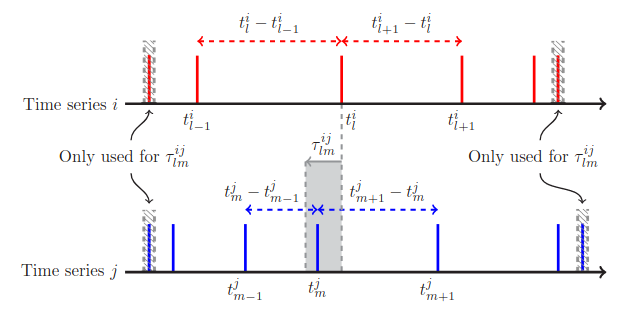
Two events \(l\) and \(m\) from timeseries \(i\) and \(j\), respectively, are considered synchronous if they occur within a certain time interval \(\tau\) which is determined from the data properties. The time interval \(\tau\) is defined as:
Thus, given an event in timeseries \(j\), the occurrences of synchronized events in \(i\) can be counted as
where \(J_{lm}^{ij}\) counts the events that match the synchronization condition. Finally, we can define the strength of event synchronization between the timeseries \(i\) and \(j\) by
In the usual case, when the timeseries are not fully synchronized, \(0 \le Q_{ij}^{ES} \le 1\), and total or absent synchronization correspond to \(Q_{ij}^{ES} = 1\) or \(Q_{ij}^{ES} = 0\), respectively. To generate an undirected network from a set of timeseries, we can consider the values \(Q_{ij}^{ES}\) as the coefficients of a square symmetric matrix \(Q^{ES}\). It should be noted that fully synchronized time series will adapt a value of \(Q_{ii}^{ES} = Q_{jj}^{ES} = 1\).
The advantage of ES is that no parameters, such as a delay specification between the two timeseries, has to selected a priori.
Event Coincidence Analysis (ECA)
In contrast, ECA incorporates static (global) coincidence intervals. For a chosen tolerance interval \(\Delta T\), an instantaneous event coincidence between two events \(t_{m}^{j} < t_{l}^{i}\) is defined by the condition \(0 \leq t_{l}^{i} - t_{m}^{j} \leq \Delta T\), and is generalized to a lagged event coincidence via a time lag \(\tau \ge 0\) on timeseries \(i\). The fundamental idea is illustrated by the picture below (Odenweller et al., 2020):
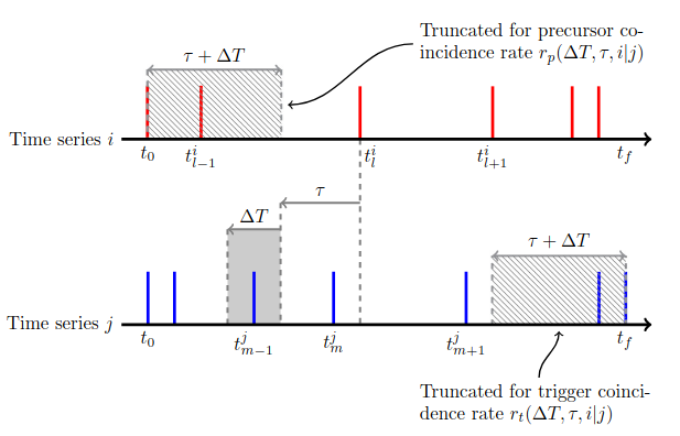
When computing the coincidence rate with ECA, the precursor and trigger event coincidence rates should be distinguished. The former refers to events in \(i\) that precede all events in \(j\), and the latter referes to events in \(j\) that precede at least one event in \(i\). More precisely, the precursor event coincidence rate is defined as
and the trigger event coincidence rate as
For details on the calculation of \(s_i', s_j''\), consult Odenweller et al. (2020). By changing the indices in the precursor or trigger rate, one obtains the opposite rates, e.g., \(r_t(j|i; \Delta T, \tau)\). Therefore, the ECA yields a total of four coincidence rates.
By computing the mean or the maximum of the two directed trigger coincidence rates \(r_t(i|j; \Delta T,\tau)\) and \(r_t(j|i;\Delta;T,\tau)\), one arrives at the degree of event synchrony \(Q_{ij}^{ECA, mean}\) or \(Q_{ij}^{ECA, max}\), which can be used as a statistical measure of uni- or bidirectional dependency.
ES/ECA for Simple Random Event Series
pyunicorn provides a class for ES and ECA. In addition, a method is included for the generation of binary event series from continuous timeseries data. First, we import the necessary packages.
[1]:
import numpy as np
from pyunicorn.eventseries import EventSeries
Input: Event Matrix
Next, we initialize the EventSeries class with a toy event matrix, in which the first axis represents the timesteps and the second axis covers the variables. Each variable at a specific timestep is either 1 if an event occurred or 0 if it did not.
[2]:
series = np.array([[0, 0],
                   [1, 1],
                   [0, 0],
                   [1, 1],
                   [0, 0],
                   [0, 0],
                   [1, 0],
                   [0, 1],
                   [0, 0],
                   [0, 0]])

ev = EventSeries(series, taumax=1)
print(ev)
EventSeries: 2 variables, 10 timesteps, taumax: 1.0, lag: 0.0
Caution: The argument taumax represents the maximum time difference \(\Delta T\) between two events that are to be considered synchronous. For ES, using the default taumax=np.inf is sensible because of its dynamic coincidence interval, whereas for ECA, a finite taumax needs to be specified.
For variables \(X,Y\), the return values of the synchronization analysis methods are:
ES: \(\left( Q^{ES}_{XY},\, Q^{ES}_{YX} \right)\)
ECA: \(\left( r_p(Y|X),\, r_t(Y|X),\, r_p(X|Y),\, r_t(X|Y) \right)\).
[3]:
print(ev.event_synchronization(*series.T))
print(ev.event_coincidence_analysis(*series.T, taumax=1))
(0.5, 0.5)
(0.5, 1.0, 1.0, 1.0)
Input: Timeseries
If the input data is not provided as an event matrix, the constructor tries to generate one from continuous time series data using the make_event_matrix() method. Therefore, the argument threshold_method needs to be specified along with the argument threshold_values. threshold_method can be 'quantile', 'value', or a 1D Numpy array with entries 'quantile' or 'value' for each variable. If 'value' is selected, one has to specify a number lying in the range of the
array; for 'quantile', a number between 0 and 1 has to be selected since it specifies the fraction of the array’s values which should be included in the event matrix. Additionally, one can specify the argument threshold_type, if the threshold should be applied 'above' or 'below' the specified threshold_method.
Here is a simple example for finding the synchrony between two continuous time series variables:
[4]:
series = (10 * np.random.rand(10, 2)).astype(int)
ev = EventSeries(series, threshold_method='quantile',
                 threshold_values=0.5, threshold_types='below', taumax=1)
print(series); print(ev)
[[8 7]
 [0 3]
 [2 5]
 [9 7]
 [3 6]
 [9 9]
 [8 1]
 [9 2]
 [8 8]
 [3 5]]
EventSeries: 2 variables, 10 timesteps, taumax: 1.0, lag: 0.0
[5]:
print("ES:", ev.event_synchronization(*series.T))
print("ECA:", ev.event_coincidence_analysis(*series.T, taumax=1))
# only compute the precursor event coincidence rates
print("ECA[p]:", ev._eca_coincidence_rate(*series.T, window_type='advanced'))
ES: (0.46770717334674267, 0.46770717334674267)
ECA: (1.0, 1.0, 1.0, 1.0)
ECA[p]: (1.0, 1.0)
Output: Event Series Measure / Functional Network
The event_series_analysis() method, with its argument method set to ES or ECA, can be used to construct a measure of dependence (functional network) as described in the introduction. Such matrices can then be subjected to complex network theory methods as a part of non-linear timeseries analysis, see Tutorial: Recurrence Networks.
The return value is a \(N\!\times\! N\) matrix, where \(N\) is the number of variables. For detailed information on the calculation of the matrix and the required arguments, please consult the API documentation.
[6]:
matrix_ES = ev.event_series_analysis(method='ES')
print("ES:"); print(matrix_ES)
matrix_ECA = ev.event_series_analysis(method='ECA', symmetrization='mean', window_type='advanced')
print("ECA:"); print(matrix_ECA)
ES:
[[0.         0.20412415]
 [0.20412415 0.        ]]
ECA:
[[0.         0.41666667]
 [0.41666667 0.        ]]
Significance Level Calculations
The signifcance levels of event synchronization can also be calculated using pyunicorn. The methods _empirical_percentiles() and event_analysis_significance() respectively estimate the \(p\)-values via a Monte Carlo approach and the signifcance levels (\(1 - p\)) via a Poisson process. For detailed information please consult the API documentation.
[7]:
print("MC[ES]:")
print(ev._empirical_percentiles(method='ES', n_surr=int(1e4)))
print("MC[ECA]:")
print(ev._empirical_percentiles(method='ECA', n_surr=int(1e4),
                                symmetrization='mean', window_type='advanced'))
print("Poisson[ES]:")
print(ev.event_analysis_significance(method='ES', n_surr=int(1e4)))
print("Poisson[ECA]:")
print(ev.event_analysis_significance(method='ECA', n_surr=int(1e4),
                                     symmetrization='mean', window_type='advanced'))
MC[ES]:
[[0.     0.2726]
 [0.271  0.    ]]
MC[ECA]:
[[0.     0.0519]
 [0.0519 0.    ]]
Poisson[ES]:
[[0.     0.2782]
 [0.2785 0.    ]]
Poisson[ECA]:
[[0.     0.0516]
 [0.0516 0.    ]]
ES/ECA for Generating a Climate Network
A possible further application of ES and ECA is the generation of climate networks from the event series measures above, and is implemented in the EventSeriesClimateNetwork class.
Note: If more general applications of event series networks are desired, use the EventSeries class together with the Network class.
[8]:
from pyunicorn.core import Data
from pyunicorn.climate.eventseries_climatenetwork import EventSeriesClimateNetwork
We shall use the small test climate dataset provided by Data.
[9]:
data = Data.SmallTestData()
print(data); print()
print(data.observable())
Data: 6 grid points, 60 measurements.
Geographical boundaries:
         time     lat     lon
   min    0.0    0.00    2.50
   max    9.0   25.00   15.00

[[ 0.00000000e+00  1.00000000e+00  1.22464680e-16 -1.00000000e+00
  -2.44929360e-16  1.00000000e+00]
 [ 3.09016994e-01  9.51056516e-01 -3.09016994e-01 -9.51056516e-01
   3.09016994e-01  9.51056516e-01]
 [ 5.87785252e-01  8.09016994e-01 -5.87785252e-01 -8.09016994e-01
   5.87785252e-01  8.09016994e-01]
 [ 8.09016994e-01  5.87785252e-01 -8.09016994e-01 -5.87785252e-01
   8.09016994e-01  5.87785252e-01]
 [ 9.51056516e-01  3.09016994e-01 -9.51056516e-01 -3.09016994e-01
   9.51056516e-01  3.09016994e-01]
 [ 1.00000000e+00  1.22464680e-16 -1.00000000e+00 -2.44929360e-16
   1.00000000e+00  3.67394040e-16]
 [ 9.51056516e-01 -3.09016994e-01 -9.51056516e-01  3.09016994e-01
   9.51056516e-01 -3.09016994e-01]
 [ 8.09016994e-01 -5.87785252e-01 -8.09016994e-01  5.87785252e-01
   8.09016994e-01 -5.87785252e-01]
 [ 5.87785252e-01 -8.09016994e-01 -5.87785252e-01  8.09016994e-01
   5.87785252e-01 -8.09016994e-01]
 [ 3.09016994e-01 -9.51056516e-01 -3.09016994e-01  9.51056516e-01
   3.09016994e-01 -9.51056516e-01]]
[10]:
climate_ES = EventSeriesClimateNetwork(
    data, method='ES', taumax=16.0,
    threshold_method='quantile', threshold_values=0.8, threshold_types='above')
print(climate_ES)
Extracting network adjacency matrix by thresholding...
Setting area weights according to type surface ...
Setting area weights according to type surface ...
EventSeriesClimateNetwork:
EventSeries: 6 variables, 10 timesteps, taumax: 16.0, lag: 0.0
ClimateNetwork:
GeoNetwork:
SpatialNetwork:
Network: directed, 6 nodes, 0 links, link density 0.000.
Geographical boundaries:
         time     lat     lon
   min    0.0    0.00    2.50
   max    9.0   25.00   15.00
Threshold: 0
Local connections filtered out: False
Type of event series measure to construct the network: directedES
[11]:
climate_ECA = EventSeriesClimateNetwork(
    data, method='ECA', taumax=16.0,
    threshold_method='quantile', threshold_values=0.8, threshold_types='above')
print(climate_ECA)
Extracting network adjacency matrix by thresholding...
Setting area weights according to type surface ...
Setting area weights according to type surface ...
EventSeriesClimateNetwork:
EventSeries: 6 variables, 10 timesteps, taumax: 16.0, lag: 0.0
ClimateNetwork:
GeoNetwork:
SpatialNetwork:
Network: directed, 6 nodes, 0 links, link density 0.000.
Geographical boundaries:
         time     lat     lon
   min    0.0    0.00    2.50
   max    9.0   25.00   15.00
Threshold: 0
Local connections filtered out: False
Type of event series measure to construct the network: directedECA